Difference between revisions of "Exploring the Hydrological Tools in QGIS"
m (clarifying that this tutorial mostly uses SAGA tools, but from the QGIS interface) |
|||
| (106 intermediate revisions by 8 users not shown) | |||
| Line 1: | Line 1: | ||
== Purpose == |
== Purpose == |
||
The purpose of this Wiki tutorial is to demonstrate and explore various |
The purpose of this Wiki tutorial is to demonstrate and explore various tools used for hydrological analyses using QGIS, concentrating on the included SAGA toolbox. The objective of this tutorial is to provide instructions on how to use digital elevation models (DEM) for extracting channel networks, delineating watersheds and defining a catchment area. Other open source software that can be used for hydrological analyses are ILWIS, and SAGA GIS, as demonstrated in a tutorial created in 2013, [https://dges.carleton.ca/CUOSGwiki/index.php/Exploring_Hydrological_Analyses_using_SAGA_GIS Exploring Hydrological Analyses using SAGA GIS] and another in 2014, [https://dges.carleton.ca/CUOSGwiki/index.php/Exploring_Hydrological_Analyses_using_ILWIS Exploring Hydrological Analyses using ILWIS]. |
||
== Introduction == |
== Introduction == |
||
Hydrological analysis tools are important resources and are used in a variety of programs to define how the geographic range of an area interacts with water. Hydrological |
Hydrological analysis tools are important resources and are used in a variety of programs to define how the geographic range of an area interacts with water. Hydrological analysis can aid researchers and emergency personnel in identifying the source and pathway of groundwater, delineating watersheds and identifying communities prone to flooding conditions [http://gracilis.carleton.ca/CUOSGwiki/index.php/Exploring_the_Hydrological_Tools_in_QGIS#Literature_Cited (Sui et. al., 2011, Mani et al., 2014)]. A variety of programs can be used to perform hydrological analyses including ARCGIS, ILWIS and SAGA GIS. This tutorial will give instructions on using QGIS, a Free and Open Source Software for Geospatial Data (FOSS4G), for hydrogeological analyses. QGIS is an open source geographic information system that runs on various platforms including Windows, Mac OS and Linux. Using a digital elevation model of the West Ottawa region, and another of Killarney Provincial Park, we will demonstrate and explore hydrogeology toolsets offered by QGIS. |
||
== Materials and methods == |
== Materials and methods == |
||
| Line 10: | Line 10: | ||
=== Data and available platforms === |
=== Data and available platforms === |
||
QGIS is a free and open source geographic information system. The current version of QGIS |
QGIS is a free and open source geographic information system. The current version of QGIS as of this tutorial revision was 3.14.16 ‘Pi,’ released on September 11th, 2020. When downloading the software, it is usually best to download the long term release, as it is the most stable; this would be version 3.10 at the time this was written. QGIS is available for a variety of platforms including Windows, Mac OS, Linux and Android. Various releases for download can be found at [http://www.qgis.org/en/site/forusers/download.html the QGIS website]. Some images show previous versions of QGIS, but instructions will be given for the current version; images of windows and menus may differ relative to your version of QGIS. |
||
Digital elevation models (DEM) are used for hydrological analyses. DEMs can be generated using point data sets from elevation data or from aerial imagery using remotely sensed data (NRCAN, 2013). Downloading a point data set would generally require interpolation of the data to create a DEM. Interpolation of a DEM will not be discussed in this tutorial. Instead, we will explore the hydrological toolset using a DEM that has previously been interpolated. |
Digital elevation models (DEM) are used for hydrological analyses. DEMs can be generated using point data sets from elevation data or from aerial imagery using remotely sensed data [http://gracilis.carleton.ca/CUOSGwiki/index.php/Exploring_the_Hydrological_Tools_in_QGIS#Literature_Cited (NRCAN, 2013)]. Downloading a point data set would generally require interpolation of the data to create a DEM. Interpolation of a DEM will not be discussed in this tutorial. Instead, we will explore the hydrological toolset using a DEM that has previously been interpolated. |
||
Often, DEM datasets that are already interpolated can be quite large, so if you are looking to analyze a large area, it might be best to find elevation point data, and interpolate them yourself. [https://dges.carleton.ca/CUOSGwiki/index.php/Creating_IDW_and_Spline_Interpolation_Maps_Using_QGIS Here is a CUOSGWiki tutorial on how to interpolate elevation point data]. And [https://www.qgistutorials.com/en/docs/interpolating_point_data.html#:~:text=QGIS%20interpolation%20supports%20Triagulated%20Irregular,as%20mineral%20concentrations%2C%20populations%20etc. here is another QGIS tutorial on interpolation]. |
|||
| ⚫ | A DEM of the southeastern quadrant of the outskirts of Ottawa, Ontario was used for the purpose of this tutorial. Data |
||
| ⚫ | A DEM of the southeastern quadrant of the outskirts of Ottawa, Ontario was used for the purpose of this tutorial. Data were obtained from the [https://library.carleton.ca/find/gis GIS Library of Carleton University] using a 3-dimensional raster data set from the Ontario Ministry of Natural Resources. The data capture terrain elevations and cover the province of Ontario with a cell resolution of 30 cm. |
||
Additional data sources can be found from Natural Resources Canada, Geogratis and from the provincial website of Ontario. |
|||
A DEM of Killarney Provincial Park and surrounding areas was also used in certain cases. Data were obtained from [[http://geo1.scholarsportal.info/#r/details/_uri@=60f2fde2-b1f0-4a1c-ac89-acc32984f614 Scholars Geoportal]], which is accessible to Carleton University students and staff. It is a 3-dimensional raster data set which captures terrain elevations with a cell resolutions of 20 metres. |
|||
Additional data sources can be found from [http://www.nrcan.gc.ca/home Natural Resources Canada], [https://geogratis.gc.ca/ Geogratis] and from the [https://www.ontario.ca/ministry-natural-resources-and-forestry Ontario Ministry of Natural Resources.] [https://library.carleton.ca/find/gis/contours-and-elevation-data Macodrum Library is also a valuable tool for finding elevation data,] they provide links to many resources, some of which are restricted to Carleton students and faculty, but many are freely accessible. |
|||
---- |
---- |
||
=== Getting started === |
=== Getting started === |
||
It is very important to create a working directory where you will keep all your data and progress files. After opening QGIS, create a new project, and save it to your working directory. |
|||
Import your DEM dataset by clicking on the “add raster tool” (Red arrow) and choosing the data in your workplace. Note: The file must be in raster format; for example, .GRID, .tiff, .rst. |
|||
Import your DEM dataset by clicking on the “Layer" tab at the top of the menu > add layer > add raster layer > click on the '...' button next to the empty field next to 'raster dataset(s)' > select your raster file > add |
|||
| ⚫ | |||
''Note: The file must be in a raster format; for example, .GRID, .tiff, .rst.'' |
|||
''Figure 1. QGIS interface. Importing a DEM dataset using the import raster tool.'' |
|||
---- |
---- |
||
=== |
=== Set projection information for your DEM === |
||
Assigning a projection to your DEM enables it to be properly displayed and analyzed. To |
Assigning a projection to your DEM enables it to be properly displayed and analyzed. To set the projection for your DEM in QGIS, follow the instructions below. |
||
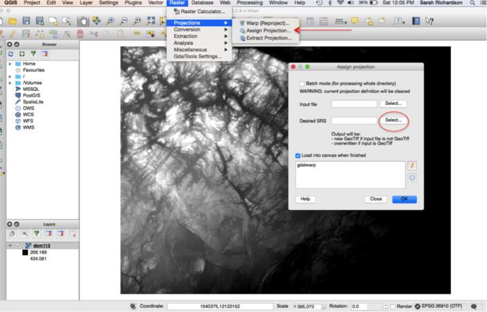
1. Click Raster > Projection > Assign Projection (Figure 2) |
1. Click Raster > Projection > Assign Projection (Figure 2) |
||
| Line 38: | Line 40: | ||
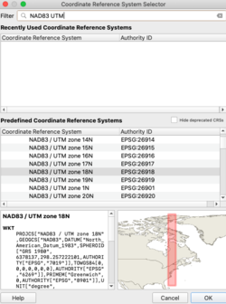
2. The Assign Projection window will appear > Click select, Desired SRS > Choose desired coordinate system and click > OK (Figure 3) |
2. The Assign Projection window will appear > Click select, Desired SRS > Choose desired coordinate system and click > OK (Figure 3) |
||
3. For the purpose of this tutorial we will be using NAD83, UTM zone |
3. For the purpose of this tutorial we will be using NAD83, UTM zone 18N |
||
4. Right |
4. Right click over your DEM layer > Properties > General > Coordinate reference system. |
||
Here is where you can verify the projected coordinate system applied to your DEM layer. |
Here is where you can verify the projected coordinate system applied to your DEM layer. |
||
5. Reclassify your DEM > Right |
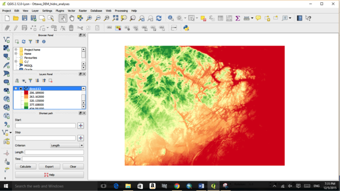
5. Reclassify your DEM > Right click over your DEM layer > Properties > Symbology > Band Rendering > Render Type > Choose Single Band Pseudocolor > Classify > Click OK (Figure 4). |
||
Reclassifying the DEM may help you have a better understanding of the data you are working with. |
|||
[[File:Projecting1.png|700px]] |
[[File:Projecting1.png|700px]] |
||
| Line 62: | Line 65: | ||
QGIS has an extensive set of tools available for hydrological analyses located in the hydrology toolbox. To access the toolbox, click on: |
QGIS has an extensive set of tools available for hydrological analyses located in the hydrology toolbox. To access the toolbox, click on: |
||
*Processing Tab > Toolbox > |
*Processing Tab > Toolbox > SAGA > Terrain Analysis: Hydrology. |
||
When opening ''Terrain Analysis - Hydrology'', you will see a long list of different tools, some are very similar and it may be hard to know which to use and for what. Because the tools are part of SAGA, there is no help tab explaining how and why to use the tools. Therefore, we have created short descriptions for each tool assessed during this tutorial for additional information. |
|||
| ⚫ | |||
''Figure 5. Example of no available help for selected tools.'' |
|||
| Line 75: | Line 74: | ||
'''''Description''''' |
'''''Description''''' |
||
*A catchment area is otherwise considered a drainage basin. The basin is |
*A catchment area is otherwise considered a drainage basin. The basin is where water flows over topographic terrain and consists of water runoff into surrounding rivers, streams and lakes. [http://gracilis.carleton.ca/CUOSGwiki/index.php/Exploring_the_Hydrological_Tools_in_QGIS#Literature_Cited (Wagener et al. 2007)]. |
||
'''''Parameters''''' |
'''''Parameters''''' |
||
| Line 82: | Line 81: | ||
*Method > Choose one model to apply to the DEM data layer |
*Method > Choose one model to apply to the DEM data layer |
||
There are five methods to choose from when delineating a catchment area from a DEM. |
There are five methods to choose from when delineating a catchment area from a DEM. |
||
*[0] Deterministic 8 (D8) |
*[0] Deterministic 8 (D8) |
||
''This is the classical method in which water flow moves from the center of one |
''This is the classical method in which water flow moves from the center of one cell to the center of one of the cells surrounding the first cell. This restricts the flow direction to multiples of 45 using 8 flow directions. [http://gracilis.carleton.ca/CUOSGwiki/index.php/Exploring_the_Hydrological_Tools_in_QGIS#Literature_Cited (O’Callaghan et al. 1984)].'' |
||
*[1] Rho 8 |
*[1] Rho 8 |
||
''This method uses an algorithm to randomly assign the direction of flow to downslope neighbouring cells depending on the degree of slope of the surrounding neighboring cells. Cells surrounding the central cell are weighted according to the degree of slope and the flow is assigned depending on the calculated weighting (Wainwright et al. 2013)'' |
''This method uses an algorithm to randomly assign the direction of flow to downslope neighbouring cells depending on the degree of slope of the surrounding neighboring cells. Cells surrounding the central cell are weighted according to the degree of slope and the flow is assigned depending on the calculated weighting. [http://gracilis.carleton.ca/CUOSGwiki/index.php/Exploring_the_Hydrological_Tools_in_QGIS#Literature_Cited (Wainwright et al. 2013)]'' |
||
*[2] Braunschweiger Reliefmodell |
*[2] Braunschweiger Reliefmodell |
||
''This method uses an algorithm to determine multiple flow |
''This method uses an algorithm to determine multiple flow directions. This model allows for flow to disperse to multiple, adjacent cells downslope from the central cell. The model restricts the flow to three cells, thus limiting the total flow dispersion of the DEM. [http://gracilis.carleton.ca/CUOSGwiki/index.php/Exploring_the_Hydrological_Tools_in_QGIS#Literature_Cited (Buchanan et al., 2014)].'' |
||
*[3] Deterministic Infinity |
*[3] Deterministic Infinity |
||
''This model delineates water flow from one cell to two surrounding cells. The model considered a bi-dimensional flow pattern and is the recommended model for reducing the limitations of the D8 model. (StackExchange, 2011).'' |
''This model delineates water flow from one cell to two surrounding cells. The model considered a bi-dimensional flow pattern and is the recommended model for reducing the limitations of the D8 model. [http://gracilis.carleton.ca/CUOSGwiki/index.php/Exploring_the_Hydrological_Tools_in_QGIS#Literature_Cited (StackExchange, 2011)].'' |
||
*[4] Multiple Flow Direction |
*[4] Multiple Flow Direction |
||
''This model assumes that flow occurs in all directions downslope from any given point. (Wolock et al. 1995).'' |
''This model assumes that flow occurs in all directions downslope from any given point. [http://gracilis.carleton.ca/CUOSGwiki/index.php/Exploring_the_Hydrological_Tools_in_QGIS#Literature_Cited (Wolock et al. 1995)].'' |
||
*[5] Multiple Triangular Flow Direction |
*[5] Multiple Triangular Flow Direction |
||
''This method avoids unrealistic flow dispersion on planar or concave slopes. This model allows for flow to disperse into one or two downslope cells, thus |
''This method avoids unrealistic flow dispersion on planar or concave slopes. This model allows for flow to disperse into one or two downslope cells, thus allowing for multiple flow directions. [http://gracilis.carleton.ca/CUOSGwiki/index.php/Exploring_the_Hydrological_Tools_in_QGIS#Literature_Cited (Seibert et. al., 2007)].'' |
||
*Catchment Area > Specify the name for the output |
*Catchment Area > Specify the name for the output layer |
||
| Line 115: | Line 116: | ||
'''''Description''''' |
'''''Description''''' |
||
*A channel network is otherwise considered a drainage network of water flow over terrain. The resulting map will demonstrate pixels with a TRUE value where flow drains |
*A channel network is otherwise considered a drainage network of water flow over terrain. The resulting map will demonstrate pixels with a TRUE value where flow drains with all pixels having no drainage will result in the pixels having a FALSE value. |
||
'''Parameters''' |
'''Parameters''' |
||
| Line 129: | Line 130: | ||
*Initiation Threshold > Insert desired threshold value |
*Initiation Threshold > Insert desired threshold value |
||
''The threshold value is the cell value required for flow to be considered TRUE in the drainage network. Adjusting the threshold value will alter the resulting drainage network because all other cells that do not meet the minimum threshold value will be considered FALSE. Increasing the threshold will result in a sparse network and decreasing the threshold will result in a dense channel network.'' |
''The threshold value is the cell value required for flow to be considered TRUE in the drainage network. Adjusting the threshold value will alter the resulting drainage network because all other cells that do not meet the minimum threshold value will be considered FALSE. Increasing the threshold will result in a sparse channel network and decreasing the threshold will result in a dense channel network.'' |
||
*Divergence (optional) > Insert optional divergence layer |
*Divergence (optional) > Insert optional divergence layer |
||
| Line 150: | Line 151: | ||
'''''Description''''' |
'''''Description''''' |
||
*Watershed basins are sub-basins determined for water flow using the channel network of the DEM |
*Watershed basins are sub-basins determined for water flow using the channel network of the DEM being analyzed [http://gracilis.carleton.ca/CUOSGwiki/index.php/Exploring_the_Hydrological_Tools_in_QGIS#Literature_Cited (Trenhaile, 2010)]. |
||
'''''Parameters''''' |
'''''Parameters''''' |
||
| Line 168: | Line 169: | ||
To access the Hydrology SAGA Toolbox in QGIS follow the below instructions. |
To access the Hydrology SAGA Toolbox in QGIS follow the below instructions. |
||
*Processing > Toolbox > |
*Processing > Toolbox > SAGA > Terrain Analysis - Hydrology OR Terrain Analysis - Channels |
||
Terrain Analysis - Channels hosts the channel network tool, as well as watershed basins tool. |
|||
---- |
---- |
||
=== Filling sinks in a DEM === |
=== Filling sinks in a DEM of a large data set === |
||
In order to extract a channel network from a DEM layer, sinks need to be filled and catchment areas need to be determined. Filling sinks allows for the removal of any local depressions from your DEM layer that can cause inaccuracy when determining channel networks. The catchment area is otherwise considered flow accumulation and can be used as the threshold layer for extracting subsequent channel network. |
In order to extract a channel network from a DEM layer, sinks need to be filled and catchment areas need to be determined. Filling sinks allows for the removal of any local depressions from your DEM layer that can cause inaccuracy when determining channel networks. The catchment area is otherwise considered flow accumulation and can be used as the threshold layer for extracting subsequent channel network. |
||
Here we will use the hydrology tool ''Fill sinks xxl (Wang & Liu)''. This specific tool is best to be used on a large data set, as the default minimum slope is 0.100000, whereas ''Fill sinks (Wang & Liu)'' has a default minimum of 0.010000, and is able to create other outputs, which will be shown in ''Flow directions and watershed basins'' below. |
|||
| ⚫ | |||
2. Fill in the specified parameters (Figure 6) |
2. Fill in the specified parameters (Figure 6) |
||
*DEM > Insert DEM data layer |
*DEM > Insert DEM data layer |
||
*Minimum Slope > Adjust slope as necessary |
*Minimum Slope > Adjust slope as necessary (default is 0.100000) |
||
*Filled DEM > Specify name for output layer |
*Filled DEM > Specify name for output layer |
||
3. Reclassify DEM (Figure 7) |
3. Reclassify DEM (Figure 7) |
||
*Right click on DEM layer > Properties > |
*Right click on DEM layer > Properties > Symbology > Band Rendering > Select Render Type > Single band Pseudocolour > Classify > OK |
||
[[File:Sinks1.png|250px]] |
[[File:Sinks1.png|250px]] |
||
| Line 197: | Line 204: | ||
=== Flow directions and watershed basins === |
=== Flow directions and watershed basins === |
||
Flow direction is the main direction of water run-off over the |
Flow direction is the main direction of water run-off over the geographic area of interest. Flow is determined with the algorithm differentiating where a given pixel would go depending on elevation and cell height values. Watershed basins are sub-basins (polygons) depicting where water would accumulate in different areas of the DEM. |
||
| ⚫ | |||
*Chose the advanced interface, SAGA algorithms because QGIS Geoalgorithms would not work |
|||
1. Click on Processing > Toolbox > SAGA > Terrain Analysis: Hydrology > Fill Sinks (Wang & Liu, Figure 8) |
|||
| ⚫ | |||
| ⚫ | |||
2. Fill in the specified parameters |
2. Fill in the specified parameters |
||
| Line 212: | Line 217: | ||
*Flow Directions > Specify name for output layer |
*Flow Directions > Specify name for output layer |
||
*Watershed Basins > Specify name for output layer |
*Watershed Basins > Specify name for output layer |
||
3. Reclassify DEM |
|||
*Right click on DEM layer > Properties > Symbology > Band Rendering > Select Render Type > Single band Pseudocolour > Classify > OK |
|||
[[File:Flow1.png|400px]] |
[[File:Flow1.png|400px]] |
||
''Figure 8. Fill sinks (Wang & Liu) toolbox for flow directions and watershed basins.'' |
''Figure 8. Fill sinks (Wang & Liu) toolbox for flow directions and watershed basins.'' |
||
[[File:Filled vs original.png|800px]] |
|||
''Figure 9. Original DEM vs. Filled image using Fill sinks (Wang & Liu) with 0.01000 as the minimum slope, you can see a slight difference. (Image of Killarney Provincial Park).'' |
|||
[[File:Flow2.png|700px]] |
[[File:Flow2.png|700px]] |
||
''Figure |
''Figure 10. Resulting flow direction map of the Southeastern quadrant of Ottawa.'' |
||
[[File:Flow3.png|700px]] |
[[File:Flow3.png|700px]] |
||
''Figure |
''Figure 11. Resulting watershed basin for the Southeastern quadrant of Ottawa.'' |
||
---- |
---- |
||
=== Defining the catchment area === |
=== Defining the catchment area === |
||
A catchment area is otherwise considered a drainage basin. The basin is the where water flows over topographic terrain and consists of water runoff into surrounding rivers, streams and lakes. (Wagener et al. 2007). There are five models to choose from: Deterministic 8, Rho 8, Braunschweiger Reliefmodell, Deterministic Infinity, Multiple Flow Direction and Multiple Triangular Flow Direction. A description of each model can be reviewed under 3.4 The Hydrology Toolbox. |
A catchment area is otherwise considered a drainage basin. The basin is the where water flows over topographic terrain and consists of water runoff into surrounding rivers, streams and lakes. [http://gracilis.carleton.ca/CUOSGwiki/index.php/Exploring_the_Hydrological_Tools_in_QGIS#Literature_Cited (Wagener et al. 2007)]. There are five models to choose from: Deterministic 8, Rho 8, Braunschweiger Reliefmodell, Deterministic Infinity, Multiple Flow Direction and Multiple Triangular Flow Direction. A description of each model can be reviewed under 3.4 The Hydrology Toolbox. |
||
1. Click on Processing > Toolbox > |
1. Click on Processing > Toolbox > SAGA > Terrain Analysis: Hydrology > Catchment Area |
||
2. Fill in the specified parameters |
2. Fill in the specified parameters |
||
| Line 237: | Line 250: | ||
*Method > Choose appropriate method |
*Method > Choose appropriate method |
||
*Catchment Area > Specify name for output layer |
*Catchment Area > Specify name for output layer |
||
The rendering of this layer is not very helpful, as you can see in Figure 13. In order for it to convey more information we must use the raster calculator to calculate the logarithm of the catchment area. |
|||
To do this: |
|||
1. Click on Raster > Raster Calculator. This will open up the raster calculator |
|||
2. Click on log10 under ''operators'' > then double click on the catchment area under ''Raster Bands'' > close the parentheses > create a name for the output layer and make sure it will save in your working directory > click OK |
|||
*Your formula should look something like ''log10(CatchmentArea)'' |
|||
*After these steps, your catchment area should look something more like Figure 14. |
|||
[[File:Catch1.png|700px]] |
[[File:Catch1.png|700px]] |
||
''Figure |
''Figure 12. Catchment area tool in the Hydrology Toolbox of QGIS.'' |
||
[[File:Killarneyb4Log.png|500px]] |
|||
''Figure 13. Catchment area of Killarney Park before using raster calculator'' |
|||
[[File:Catch2.png|700px]] |
[[File:Catch2.png|700px]] |
||
''Figure |
''Figure 14. Catchment area of the Southeastern Quadrant of Ottawa using the Deterministic 8 method.'' |
||
[[File:Catch3.png|700px]] |
[[File:Catch3.png|700px]] |
||
''Figure |
''Figure 15. Catchment area of the Southeastern Quadrant of Ottawa using the Rho 8 method.'' |
||
[[File:Catch4.png|700px]] |
[[File:Catch4.png|700px]] |
||
''Figure |
''Figure 16. Catchment area of the Southeastern Quadrant of Ottawa using the Braunschweiger Reliefmodell method.'' |
||
[[File:Catch5.png|700px]] |
[[File:Catch5.png|700px]] |
||
''Figure |
''Figure 17. Catchment area of the Southeastern Quadrant of Ottawa using the Deterministic infinity method.'' |
||
[[File:Catch6.png|700px]] |
[[File:Catch6.png|700px]] |
||
''Figure |
''Figure 18. Catchment area of the Southeastern Quadrant of Ottawa using the Multiple Flow Direction method.'' |
||
[[File:Catch7.png|700px]] |
[[File:Catch7.png|700px]] |
||
''Figure |
''Figure 19. Catchment area of the Southeastern Quadrant of Ottawa using the Multiple Triangular Flow Direction method.'' |
||
---- |
---- |
||
=== Channel network of a DEM === |
=== Channel network of a DEM === |
||
A channel network is otherwise considered a drainage network of water flow over terrain. The resulting map will demonstrate pixels with a TRUE value where flow drains with all pixels |
A channel network is otherwise considered a drainage network of water flow over terrain. The resulting map will demonstrate pixels with a TRUE value where flow drains with all pixels having no drainage results in pixels having a FALSE value. Here we will demonstrate how to extract a channel network from the DEM of Ottawa using the SAGA Toolbox in the advanced processing function in QGIS. This enables us to create multiple maps using one tool. |
||
1. Processing > Toolbox |
1. Processing > Toolbox > SAGA > Terrain Analysis - Channels > Channel Network and Drainage Basins |
||
2. Fill in the specified parameters |
2. Fill in the specified parameters |
||
| Line 283: | Line 312: | ||
*Drainage Basins (shapefile) > Specify name for output layer |
*Drainage Basins (shapefile) > Specify name for output layer |
||
*Junctions (shapefile) > Specify name for output layer |
*Junctions (shapefile) > Specify name for output layer |
||
| ⚫ | |||
''Figure 19. Channel Network and Drainage Basins tool in the advanced interface processing SAGA tool box in QGIS.'' |
|||
| ⚫ | |||
''Figure 20. Drainage Basins and Channels of Southeastern Quadrant of Ottawa using the Channels and Basins SAGA tool in QGIS.'' |
|||
[[File:Channel3.png|700px]] |
|||
''Figure 21. Channels of Southeastern Quadrant of Ottawa using the Channels and Basins SAGA tool in QGIS.'' |
|||
== Conclusion == |
== Conclusion == |
||
In conclusion, we have demonstrated how to use various SAGA hydrological tools offered in the free and open source software of QGIS using a DEM of the West Ottawa region and Killarney Provincial Park. Hydrological analysis tools are an important resource for determining how the geography of any area interacts with water, and thus, have important applicability to safety, engineering and ecology perspectives. |
|||
== Literature Cited == |
== Literature Cited == |
||
Buchanan, BP., Fleming, M., Schneider, RI., Richards, BK., Archibald, J., Qui, Z., Walter, M.T., 2014. Evaluating topographic wetness indices across central New York agricultural landscapes. Hydrology Earth System Sciences, 18: 3279-3299.[https://www.researchgate.net/publication/260957994_Evaluating_topographic_wetness_indices_across_Central_New_York_agricultural_landscapes] |
|||
Maidment, D., Djokic, D., 2000. Hydrologic and Hydraulic Modeling Support with Geographic Information Systems. Environmental Systems Research Institute Inc., Redlands, California. 213pp. [https://books.google.ca/books?id=A_iTo003UUAC&pg=PA217&lpg=PA217&dq=Hydrologic+and+Hydraulic+Modeling+Support+with+Geographic+Information+Systems&source=bl&ots=2bL_f_hode&sig=yzgJxo86Khtfb9ySitOXD-AVnNE&hl=en&sa=X&ved=0ahUKEwiPyfSnrtLJAhVBHD4KHdmgCb4Q6AEILDAC#v=onepage&q=Hydrologic%20and%20Hydraulic%20Modeling%20Support%20with%20Geographic%20Information%20Systems&f=false] |
|||
O’Callaghan, JF., Mark, DM., 1984. The extraction of drainage networks from digital elevation data. Computer Vision, Graphics, and Image Processing, 28(3): 323-344. [http://www.sciencedirect.com/science/article/pii/S0734189X84800110] |
|||
Seibert, J., McGlynn, BL., 2007. A new triangular multiple flow direction algorithm for computing upslope areas from gridded digital elevation models. Water Resources Research, 43(4): doi: 10.1029/2006WR005128.[http://onlinelibrary.wiley.com/doi/10.1029/2006WR005128/abstract] |
|||
Shamsi, UM., 2005. GIS Applications for Water, Wastewater, and Stormwater Systems. CRC Press Inc., Boca Raton, Florida. 398pp. [https://books.google.ca/books?id=XiHNBQAAQBAJ&pg=PA6&lpg=PA6&dq=GIS+Applications+for+Water,+Wastewater,+and+Stormwater+Systems&source=bl&ots=IUZCoz2XWj&sig=hUIODePrP6qYS7xv0bII9lEPPMA&hl=en&sa=X&ved=0ahUKEwjE_u7mrtLJAhWKNT4KHWQZCYsQ6AEIRjAH#v=onepage&q=GIS%20Applications%20for%20Water%2C%20Wastewater%2C%20and%20Stormwater%20Systems&f=false] |
|||
StackExchange, 2011. Geographic information systems: Given a terrain, how to determine stream flow path? Retrieved on Dec 1st 2015 from [http://gis.stackexchange.com/questions/14622/given-a-terrain-how-to-draw-the-stream-flow-path.] |
|||
Trenhaile, AS., 2010. Geomorphology: A Canadian Perspective. Fourth Edition, Oxford University Press. Ontario, Canada. |
|||
Wainwright, J., Mulligan, M., 2013. Environmental Modeling: Finding Simplicity in Complexity. John Wiley & Sons, Ltd. West Sussex, UK. 496pp. [https://books.google.ca/books?id=OMrYDQGprVwC&printsec=frontcover&source=gbs_ge_summary_r&cad=0#v=onepage&q&f=false] |
|||
Wagener, T., Sivapalan, M., Troch, P., Woods, R., 2007. Catchment classification and hydrologic similarity.Geography Compass, 1(4): 901-931. [http://onlinelibrary.wiley.com/doi/10.1111/j.1749-8198.2007.00039.x/abstract] |
|||
Wolock, DM., McCabe Jr., GJ., 1995. Comparison of single and multiple flow direction algorithms for computing topographic parameters in TOPMODEL. Water Resources Research, 31(5): 1315-1324 [http://onlinelibrary.wiley.com/doi/10.1029/95WR00471/full] |
|||
Latest revision as of 11:25, 18 October 2020
Contents
- 1 Purpose
- 2 Introduction
- 3 Materials and methods
- 4 Conclusion
- 5 Literature Cited
Purpose
The purpose of this Wiki tutorial is to demonstrate and explore various tools used for hydrological analyses using QGIS, concentrating on the included SAGA toolbox. The objective of this tutorial is to provide instructions on how to use digital elevation models (DEM) for extracting channel networks, delineating watersheds and defining a catchment area. Other open source software that can be used for hydrological analyses are ILWIS, and SAGA GIS, as demonstrated in a tutorial created in 2013, Exploring Hydrological Analyses using SAGA GIS and another in 2014, Exploring Hydrological Analyses using ILWIS.
Introduction
Hydrological analysis tools are important resources and are used in a variety of programs to define how the geographic range of an area interacts with water. Hydrological analysis can aid researchers and emergency personnel in identifying the source and pathway of groundwater, delineating watersheds and identifying communities prone to flooding conditions (Sui et. al., 2011, Mani et al., 2014). A variety of programs can be used to perform hydrological analyses including ARCGIS, ILWIS and SAGA GIS. This tutorial will give instructions on using QGIS, a Free and Open Source Software for Geospatial Data (FOSS4G), for hydrogeological analyses. QGIS is an open source geographic information system that runs on various platforms including Windows, Mac OS and Linux. Using a digital elevation model of the West Ottawa region, and another of Killarney Provincial Park, we will demonstrate and explore hydrogeology toolsets offered by QGIS.
Materials and methods
Data and available platforms
QGIS is a free and open source geographic information system. The current version of QGIS as of this tutorial revision was 3.14.16 ‘Pi,’ released on September 11th, 2020. When downloading the software, it is usually best to download the long term release, as it is the most stable; this would be version 3.10 at the time this was written. QGIS is available for a variety of platforms including Windows, Mac OS, Linux and Android. Various releases for download can be found at the QGIS website. Some images show previous versions of QGIS, but instructions will be given for the current version; images of windows and menus may differ relative to your version of QGIS.
Digital elevation models (DEM) are used for hydrological analyses. DEMs can be generated using point data sets from elevation data or from aerial imagery using remotely sensed data (NRCAN, 2013). Downloading a point data set would generally require interpolation of the data to create a DEM. Interpolation of a DEM will not be discussed in this tutorial. Instead, we will explore the hydrological toolset using a DEM that has previously been interpolated.
Often, DEM datasets that are already interpolated can be quite large, so if you are looking to analyze a large area, it might be best to find elevation point data, and interpolate them yourself. Here is a CUOSGWiki tutorial on how to interpolate elevation point data. And here is another QGIS tutorial on interpolation.
A DEM of the southeastern quadrant of the outskirts of Ottawa, Ontario was used for the purpose of this tutorial. Data were obtained from the GIS Library of Carleton University using a 3-dimensional raster data set from the Ontario Ministry of Natural Resources. The data capture terrain elevations and cover the province of Ontario with a cell resolution of 30 cm.
A DEM of Killarney Provincial Park and surrounding areas was also used in certain cases. Data were obtained from [Scholars Geoportal], which is accessible to Carleton University students and staff. It is a 3-dimensional raster data set which captures terrain elevations with a cell resolutions of 20 metres.
Additional data sources can be found from Natural Resources Canada, Geogratis and from the Ontario Ministry of Natural Resources. Macodrum Library is also a valuable tool for finding elevation data, they provide links to many resources, some of which are restricted to Carleton students and faculty, but many are freely accessible.
Getting started
It is very important to create a working directory where you will keep all your data and progress files. After opening QGIS, create a new project, and save it to your working directory.
Import your DEM dataset by clicking on the “Layer" tab at the top of the menu > add layer > add raster layer > click on the '...' button next to the empty field next to 'raster dataset(s)' > select your raster file > add
Note: The file must be in a raster format; for example, .GRID, .tiff, .rst.
Set projection information for your DEM
Assigning a projection to your DEM enables it to be properly displayed and analyzed. To set the projection for your DEM in QGIS, follow the instructions below.
1. Click Raster > Projection > Assign Projection (Figure 2)
2. The Assign Projection window will appear > Click select, Desired SRS > Choose desired coordinate system and click > OK (Figure 3)
3. For the purpose of this tutorial we will be using NAD83, UTM zone 18N
4. Right click over your DEM layer > Properties > General > Coordinate reference system. Here is where you can verify the projected coordinate system applied to your DEM layer.
5. Reclassify your DEM > Right click over your DEM layer > Properties > Symbology > Band Rendering > Render Type > Choose Single Band Pseudocolor > Classify > Click OK (Figure 4). Reclassifying the DEM may help you have a better understanding of the data you are working with.
Figure 2. Assigning a projection to your DEM layer.
Figure 3. Choosing a desired coordinate system for your DEM layer.
Figure 4. Reclassification of a DEM.
The hydrology toolboxes
QGIS has an extensive set of tools available for hydrological analyses located in the hydrology toolbox. To access the toolbox, click on:
- Processing Tab > Toolbox > SAGA > Terrain Analysis: Hydrology.
When opening Terrain Analysis - Hydrology, you will see a long list of different tools, some are very similar and it may be hard to know which to use and for what. Because the tools are part of SAGA, there is no help tab explaining how and why to use the tools. Therefore, we have created short descriptions for each tool assessed during this tutorial for additional information.
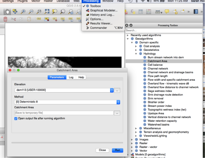
TOOLBOX A. Catchment Area
Description
- A catchment area is otherwise considered a drainage basin. The basin is where water flows over topographic terrain and consists of water runoff into surrounding rivers, streams and lakes. (Wagener et al. 2007).
Parameters
- Elevation > Insert DEM data layer
- Method > Choose one model to apply to the DEM data layer
There are five methods to choose from when delineating a catchment area from a DEM.
- [0] Deterministic 8 (D8)
This is the classical method in which water flow moves from the center of one cell to the center of one of the cells surrounding the first cell. This restricts the flow direction to multiples of 45 using 8 flow directions. (O’Callaghan et al. 1984).
- [1] Rho 8
This method uses an algorithm to randomly assign the direction of flow to downslope neighbouring cells depending on the degree of slope of the surrounding neighboring cells. Cells surrounding the central cell are weighted according to the degree of slope and the flow is assigned depending on the calculated weighting. (Wainwright et al. 2013)
- [2] Braunschweiger Reliefmodell
This method uses an algorithm to determine multiple flow directions. This model allows for flow to disperse to multiple, adjacent cells downslope from the central cell. The model restricts the flow to three cells, thus limiting the total flow dispersion of the DEM. (Buchanan et al., 2014).
- [3] Deterministic Infinity
This model delineates water flow from one cell to two surrounding cells. The model considered a bi-dimensional flow pattern and is the recommended model for reducing the limitations of the D8 model. (StackExchange, 2011).
- [4] Multiple Flow Direction
This model assumes that flow occurs in all directions downslope from any given point. (Wolock et al. 1995).
- [5] Multiple Triangular Flow Direction
This method avoids unrealistic flow dispersion on planar or concave slopes. This model allows for flow to disperse into one or two downslope cells, thus allowing for multiple flow directions. (Seibert et. al., 2007).
- Catchment Area > Specify the name for the output layer
TOOLBOX B. Channel Network
Description
- A channel network is otherwise considered a drainage network of water flow over terrain. The resulting map will demonstrate pixels with a TRUE value where flow drains with all pixels having no drainage will result in the pixels having a FALSE value.
Parameters
- Elevation > Insert DEM data layer
- Flow Direction (optional) > Insert optional flow direction layer
- Initiation Grid > Insert Catchment Area layer or desired input layer of your choice
- Initiation Type > Choose from [0] Less than, [1] Equals, or [2] Greater than
- Initiation Threshold > Insert desired threshold value
The threshold value is the cell value required for flow to be considered TRUE in the drainage network. Adjusting the threshold value will alter the resulting drainage network because all other cells that do not meet the minimum threshold value will be considered FALSE. Increasing the threshold will result in a sparse channel network and decreasing the threshold will result in a dense channel network.
- Divergence (optional) > Insert optional divergence layer
- The divergence layer is a layer that determines if flow diverges from the specified channel.
- Tracing: Max. Divergence > default = 10, adjust accordingly
- Tracing: Weight (optional) > Insert optional weighting layer for tracing network
- Min. Segment Length > default = 10, adjust accordingly
- Channel Network > Specify the name for the output layer
- Channel Direction > Specify the name for the output layer
TOOLBOX C. Watershed Basins
Description
- Watershed basins are sub-basins determined for water flow using the channel network of the DEM being analyzed (Trenhaile, 2010).
Parameters
- Elevation > Insert DEM data layer
- Channel Network > Insert channel network layer
- Sink Route (optional) > Insert optional sink route layer
- Min. Size > default = 0, adjust accordingly
- Watershed basin > Specify the name for the output layer
The hydrology SAGA Toolbox
To access the Hydrology SAGA Toolbox in QGIS follow the below instructions.
- Processing > Toolbox > SAGA > Terrain Analysis - Hydrology OR Terrain Analysis - Channels
Terrain Analysis - Channels hosts the channel network tool, as well as watershed basins tool.
Filling sinks in a DEM of a large data set
In order to extract a channel network from a DEM layer, sinks need to be filled and catchment areas need to be determined. Filling sinks allows for the removal of any local depressions from your DEM layer that can cause inaccuracy when determining channel networks. The catchment area is otherwise considered flow accumulation and can be used as the threshold layer for extracting subsequent channel network.
Here we will use the hydrology tool Fill sinks xxl (Wang & Liu). This specific tool is best to be used on a large data set, as the default minimum slope is 0.100000, whereas Fill sinks (Wang & Liu) has a default minimum of 0.010000, and is able to create other outputs, which will be shown in Flow directions and watershed basins below.
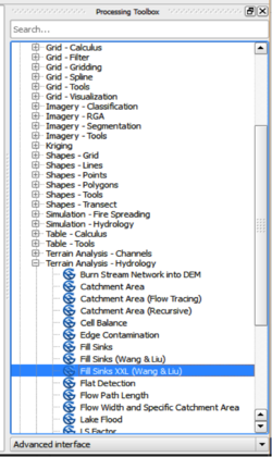
1. Processing > Toolbox > SAGA > Terrain Analysis: Hydrology > Fill Sinks xxl(Wang & Liu).
2. Fill in the specified parameters (Figure 6)
- DEM > Insert DEM data layer
- Minimum Slope > Adjust slope as necessary (default is 0.100000)
- Filled DEM > Specify name for output layer
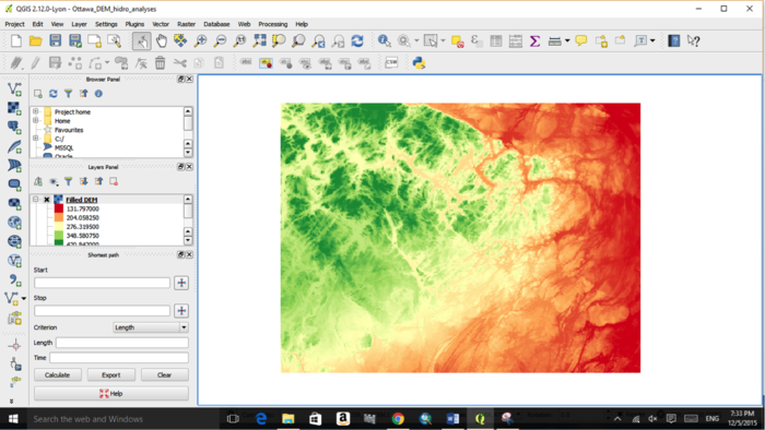
3. Reclassify DEM (Figure 7)
- Right click on DEM layer > Properties > Symbology > Band Rendering > Select Render Type > Single band Pseudocolour > Classify > OK
Figure 6. Filling sinks toolbox location for DEM.
Figure 7. Filled DEM of the southeastern quadrant of Ottawa.
Flow directions and watershed basins
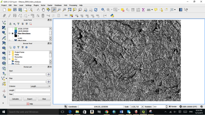
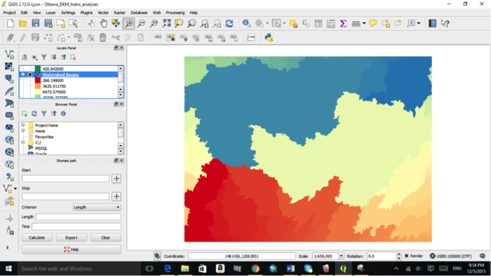
Flow direction is the main direction of water run-off over the geographic area of interest. Flow is determined with the algorithm differentiating where a given pixel would go depending on elevation and cell height values. Watershed basins are sub-basins (polygons) depicting where water would accumulate in different areas of the DEM.
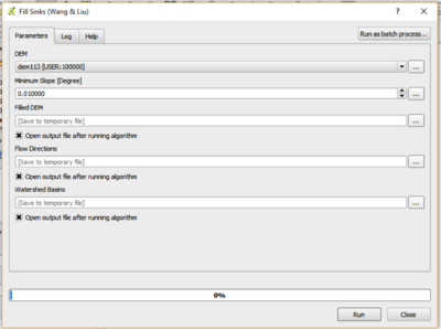
Using the Fill Sinks (Wang & Liu) tool, flow direction and watershed basins can be created while filling the sinks within the DEM.
1. Click on Processing > Toolbox > SAGA > Terrain Analysis: Hydrology > Fill Sinks (Wang & Liu, Figure 8)
2. Fill in the specified parameters
- DEM > Insert DEM Data Layer
- Min. Slope > Specify minimum slope requirement, adjust as necessary
- Filled DEM > Specify name for output layer
- Flow Directions > Specify name for output layer
- Watershed Basins > Specify name for output layer
3. Reclassify DEM
- Right click on DEM layer > Properties > Symbology > Band Rendering > Select Render Type > Single band Pseudocolour > Classify > OK
Figure 8. Fill sinks (Wang & Liu) toolbox for flow directions and watershed basins.
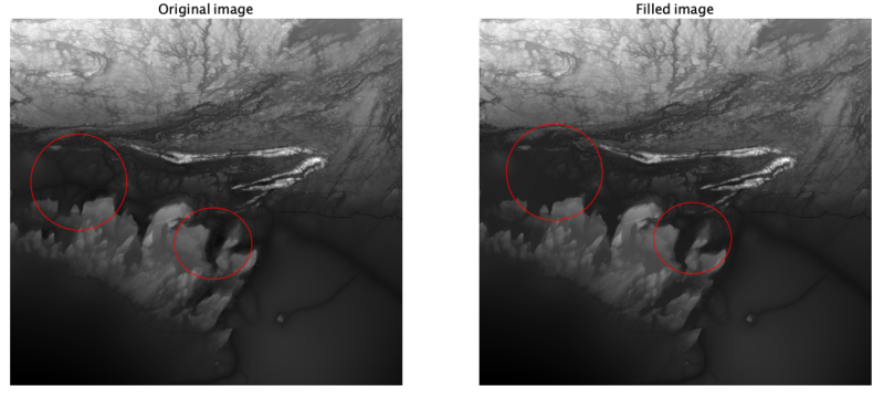
Figure 9. Original DEM vs. Filled image using Fill sinks (Wang & Liu) with 0.01000 as the minimum slope, you can see a slight difference. (Image of Killarney Provincial Park).
Figure 10. Resulting flow direction map of the Southeastern quadrant of Ottawa.
Figure 11. Resulting watershed basin for the Southeastern quadrant of Ottawa.
Defining the catchment area
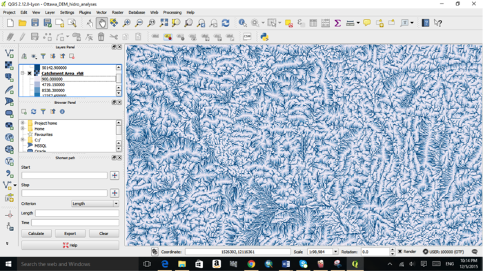
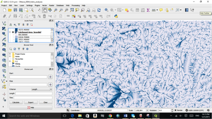
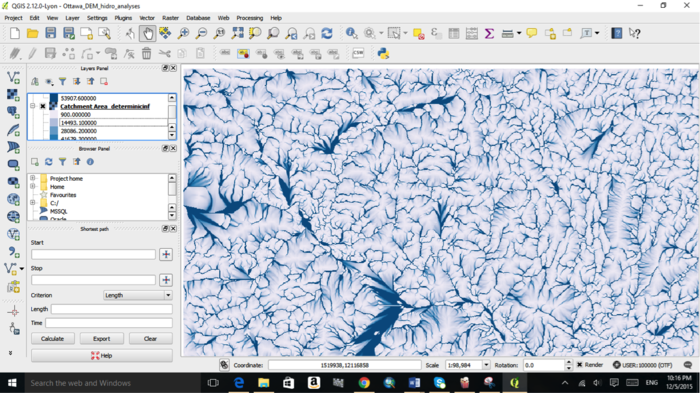
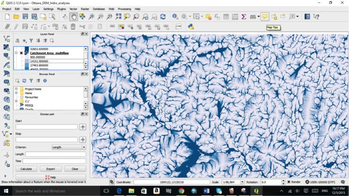
A catchment area is otherwise considered a drainage basin. The basin is the where water flows over topographic terrain and consists of water runoff into surrounding rivers, streams and lakes. (Wagener et al. 2007). There are five models to choose from: Deterministic 8, Rho 8, Braunschweiger Reliefmodell, Deterministic Infinity, Multiple Flow Direction and Multiple Triangular Flow Direction. A description of each model can be reviewed under 3.4 The Hydrology Toolbox.
1. Click on Processing > Toolbox > SAGA > Terrain Analysis: Hydrology > Catchment Area
2. Fill in the specified parameters
- Elevation > Insert DEM layer (filled DEM)
- Method > Choose appropriate method
- Catchment Area > Specify name for output layer
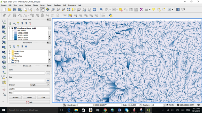
The rendering of this layer is not very helpful, as you can see in Figure 13. In order for it to convey more information we must use the raster calculator to calculate the logarithm of the catchment area.
To do this:
1. Click on Raster > Raster Calculator. This will open up the raster calculator
2. Click on log10 under operators > then double click on the catchment area under Raster Bands > close the parentheses > create a name for the output layer and make sure it will save in your working directory > click OK
- Your formula should look something like log10(CatchmentArea)
- After these steps, your catchment area should look something more like Figure 14.
Figure 12. Catchment area tool in the Hydrology Toolbox of QGIS.
Figure 13. Catchment area of Killarney Park before using raster calculator
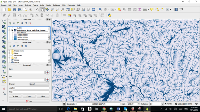
Figure 14. Catchment area of the Southeastern Quadrant of Ottawa using the Deterministic 8 method.
Figure 15. Catchment area of the Southeastern Quadrant of Ottawa using the Rho 8 method.
Figure 16. Catchment area of the Southeastern Quadrant of Ottawa using the Braunschweiger Reliefmodell method.
Figure 17. Catchment area of the Southeastern Quadrant of Ottawa using the Deterministic infinity method.
Figure 18. Catchment area of the Southeastern Quadrant of Ottawa using the Multiple Flow Direction method.
Figure 19. Catchment area of the Southeastern Quadrant of Ottawa using the Multiple Triangular Flow Direction method.
Channel network of a DEM
A channel network is otherwise considered a drainage network of water flow over terrain. The resulting map will demonstrate pixels with a TRUE value where flow drains with all pixels having no drainage results in pixels having a FALSE value. Here we will demonstrate how to extract a channel network from the DEM of Ottawa using the SAGA Toolbox in the advanced processing function in QGIS. This enables us to create multiple maps using one tool.
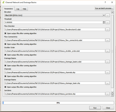
1. Processing > Toolbox > SAGA > Terrain Analysis - Channels > Channel Network and Drainage Basins
2. Fill in the specified parameters
- Elevations > Insert DEM layer (filled DEM)
- Threshold > default = 5, Insert desired threshold limit
- Flow Direction > Specify name for output layer
- Flow Connectivity > Specify name for output layer
- Strahler Order > Specify name for output layer
- Drainage Basins > Specify name for output layer
- Channels (shapefile) > Specify name for output layer
- Drainage Basins (shapefile) > Specify name for output layer
- Junctions (shapefile) > Specify name for output layer
Figure 19. Channel Network and Drainage Basins tool in the advanced interface processing SAGA tool box in QGIS.
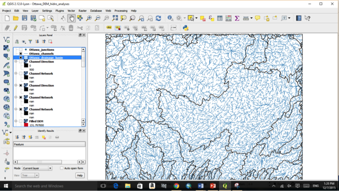
Figure 20. Drainage Basins and Channels of Southeastern Quadrant of Ottawa using the Channels and Basins SAGA tool in QGIS.
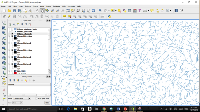
Figure 21. Channels of Southeastern Quadrant of Ottawa using the Channels and Basins SAGA tool in QGIS.
Conclusion
In conclusion, we have demonstrated how to use various SAGA hydrological tools offered in the free and open source software of QGIS using a DEM of the West Ottawa region and Killarney Provincial Park. Hydrological analysis tools are an important resource for determining how the geography of any area interacts with water, and thus, have important applicability to safety, engineering and ecology perspectives.
Literature Cited
Buchanan, BP., Fleming, M., Schneider, RI., Richards, BK., Archibald, J., Qui, Z., Walter, M.T., 2014. Evaluating topographic wetness indices across central New York agricultural landscapes. Hydrology Earth System Sciences, 18: 3279-3299.[1]
Maidment, D., Djokic, D., 2000. Hydrologic and Hydraulic Modeling Support with Geographic Information Systems. Environmental Systems Research Institute Inc., Redlands, California. 213pp. [2]
O’Callaghan, JF., Mark, DM., 1984. The extraction of drainage networks from digital elevation data. Computer Vision, Graphics, and Image Processing, 28(3): 323-344. [3]
Seibert, J., McGlynn, BL., 2007. A new triangular multiple flow direction algorithm for computing upslope areas from gridded digital elevation models. Water Resources Research, 43(4): doi: 10.1029/2006WR005128.[4]
Shamsi, UM., 2005. GIS Applications for Water, Wastewater, and Stormwater Systems. CRC Press Inc., Boca Raton, Florida. 398pp. [5]
StackExchange, 2011. Geographic information systems: Given a terrain, how to determine stream flow path? Retrieved on Dec 1st 2015 from [6]
Trenhaile, AS., 2010. Geomorphology: A Canadian Perspective. Fourth Edition, Oxford University Press. Ontario, Canada.
Wainwright, J., Mulligan, M., 2013. Environmental Modeling: Finding Simplicity in Complexity. John Wiley & Sons, Ltd. West Sussex, UK. 496pp. [7]
Wagener, T., Sivapalan, M., Troch, P., Woods, R., 2007. Catchment classification and hydrologic similarity.Geography Compass, 1(4): 901-931. [8]
Wolock, DM., McCabe Jr., GJ., 1995. Comparison of single and multiple flow direction algorithms for computing topographic parameters in TOPMODEL. Water Resources Research, 31(5): 1315-1324 [9]
